


Conditional simulation
Overview
Conditional Simulation is an advanced geostatistical technique. It is useful for assessing risk associated with an estimate. Other estimation methods, such as inverse distance weighting and ordinary kriging have a tendency to "smooth" data values. In general, the standard deviation and coefficient of variation of the block values estimated with these techniques will be less than for the data set that was used to perform the estimate. The histogram of the estimated blocks will have a higher minimum value and a lower maximum value than the histogram of the data.
Conditional simulation theory attempts to create a set of block estimates which is conditioned to simulate the histogram and other basic statistical parameters of the input data.
You will learn about:
- normal scores transformation
- conditional simulation estimation
Requirements
In order to understand this information, you should:
- be familiar with Surpac string files and block models
- know how to create and use variogram maps
- understand the concepts of anisotropy and kriging
Normal scores transformation
Conditional simulation requires the maximum sill of the variogram to be 1.0. This is achievable by first performing a normal scores transformation of the data.
Task: Perform a normal scores transformation
- Open gc_zone1_130.str in Graphics.
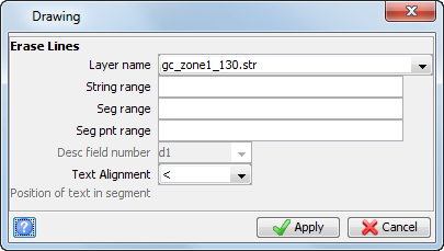
- Choose Display > Hide strings > As lines.
- Enter the information as shown, and click Apply.
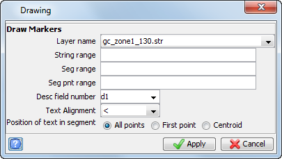
- Choose Display > Point > Markers.
- Enter the information as shown, and click Apply.
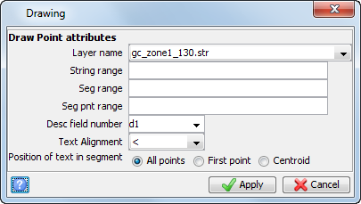
- Choose Display > Point > Attributes.
- Enter the information as shown, and click Apply.
- The D1 values are displayed.
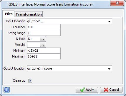
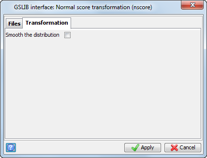
- Choose Estimation > GSLIB > Normal score transformation (nscore).
- Enter the information as shown on the two tabs of the following form, and click Apply.
- Open gc_zone1_nscore_130.str in Graphics.
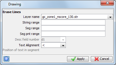
- Choose Display > Hide strings > As lines.
- Enter the information as shown, and click Apply.
- Choose Display > Point > Attributes.
- Enter the information as shown, and click Apply.
- Choose Geostatistics > Basic statistics.
- Choose File > Load data from string files.
- Enter the information as shown on each tab of the following form, and click Apply.
- Choose Display > Histogram.
- Choose Display > Normal distribution curve.
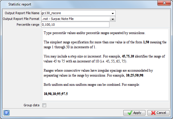
- Choose Statistics > Report.
- Enter the information as shown, and click Apply.
- Choose File > Close.
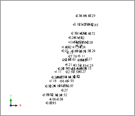
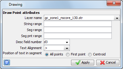
The D3 values are displayed.
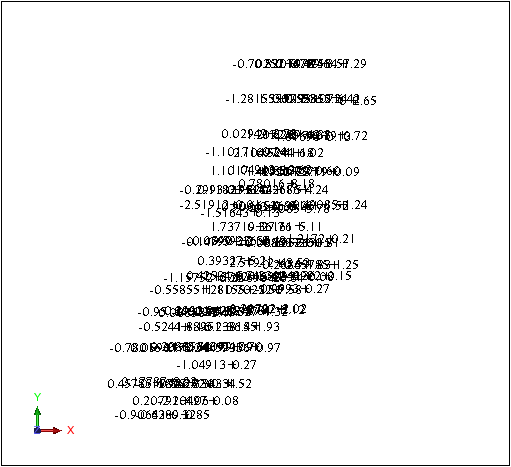
The D1 values in the output file are the same as the input data, and the D3 field contains the normal score transformed data.
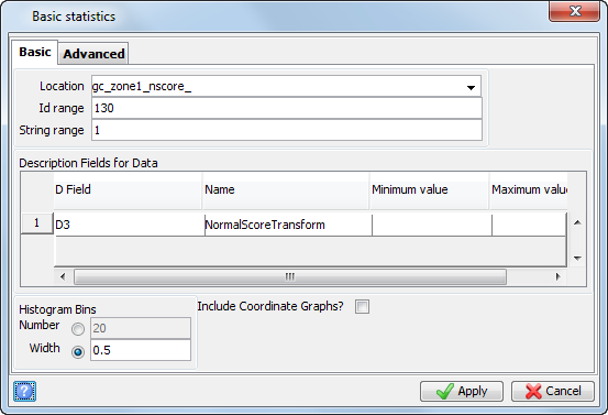
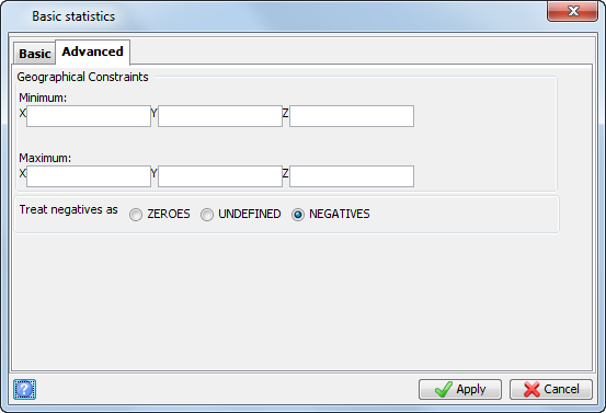
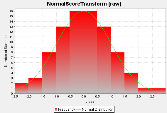
The histogram of the normal scores transformed data is very close to a normal distribution.
 Note: To see all of the steps in this task, run 2d_12a_nscore.tcl. You need to click Apply on any forms presented.
Task: Calculate anisotropy parameters for normal score transformed data
- Choose Geostatistics > Variogram modelling.
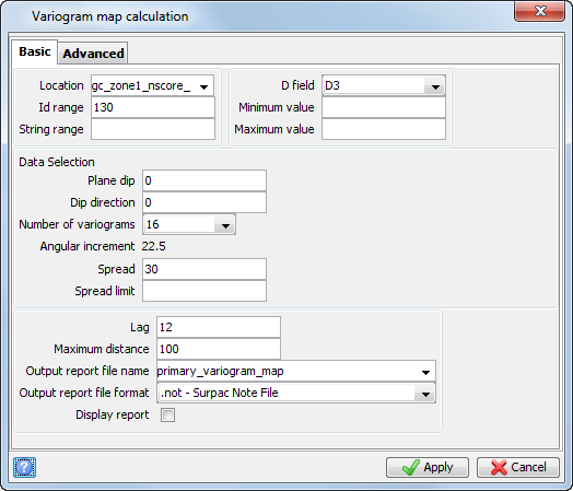
- Choose Variogram Map > New variogram map.
- Enter the information as shown and click Apply.
- Right-click and choose Tile Windows.
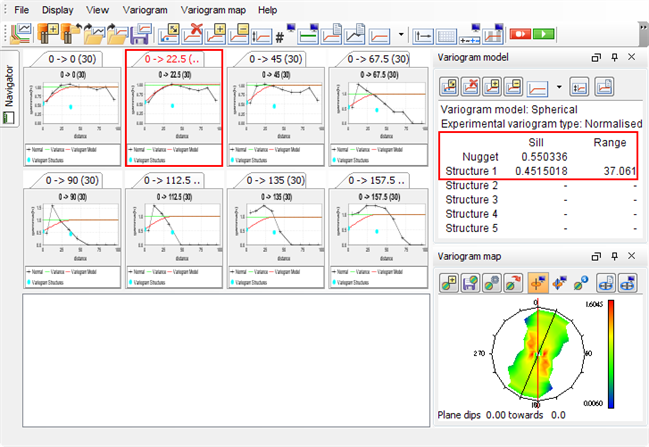
- Use the variogram map to identify the major axis, as shown.
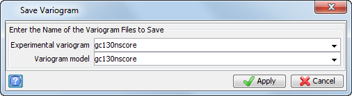
- Choose File > Save > Experimental variogram and model
- Enter the information as shown, and click Apply.
- Modify the variogram to fit it to the variogram for the semi-major axis (keep the nugget and sill the same), and note the range.
- You must document the following information for use in the conditional simulation function (SGSIM).
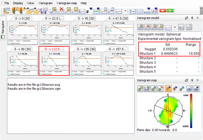
| SGSIM Parameter | Description | Value |
|---|---|---|
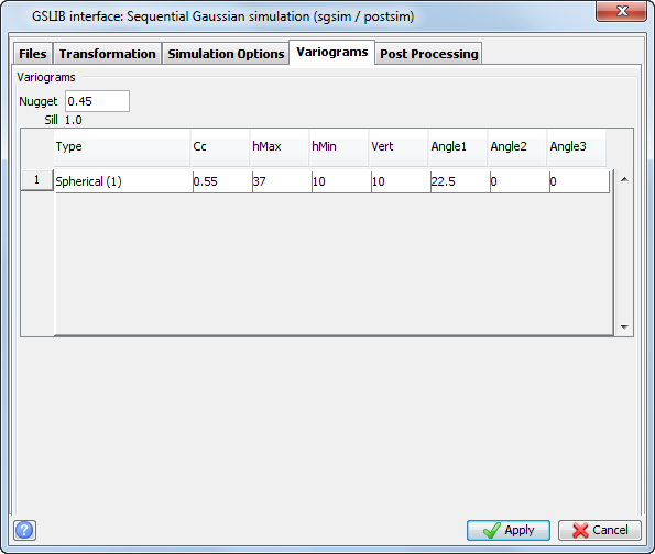
| Angle1 | Bearing of major axis | 22.5 |
| Nugget | Nugget of major axis variogram | 0.45 |
| Cc | Sill of major axis variogram | 0.55 |
| hMax | range of major axis variogram | 37 |
| hMin | range of semi-major axis variogram | 10 |
| Vert | range of minor axis variogram | 10(=hMin) |
Task: Perform conditional simulation using SGSIM
- Run 2d_12c_create_sim_model.tcl to create (or recreate) the model gc_130simulation.mdl and constraints sim_orezone1.con and sim_orezone2.con.
- Open gc_130simulation.mdl.
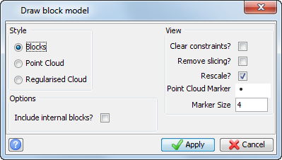
- Choose Display > Display block model.
- Enter the information as shown, and click Apply.
- Choose Constraints > New graphical constraint.
- Enter the information as shown, and click Apply.
- Choose Estimation > GSLIB > Sequential Gaussian simulation (sgsim / postsim).
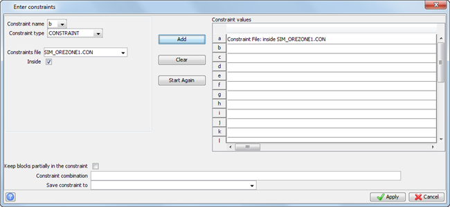
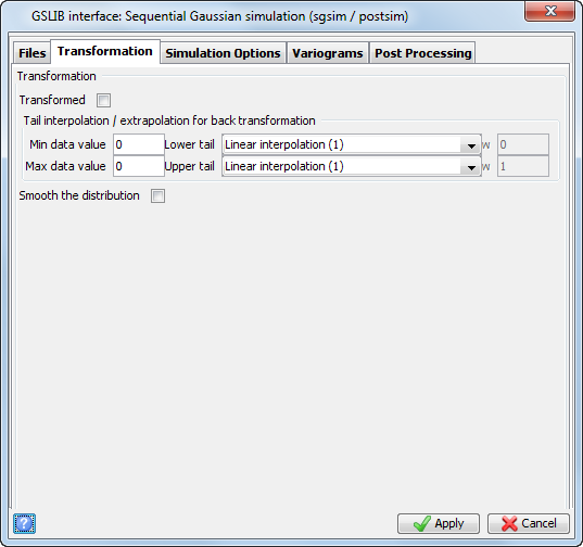
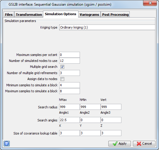
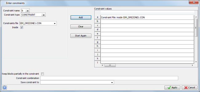
- Enter the information as shown on the five tabs of this form, and the Enter constraints form, and click Apply.
- On the Verify creating of file form, click Yes.
- Choose Attributes > View attributes for one block.
- Select a block.
- Click Apply.
- Choose Block model > Save.
- Choose Block model > Close.
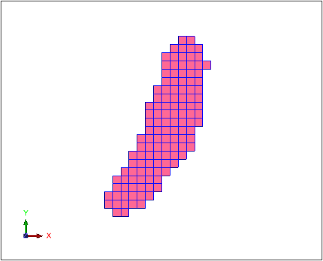
The constrained model is displayed.
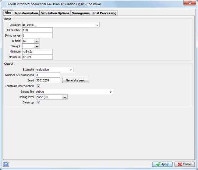
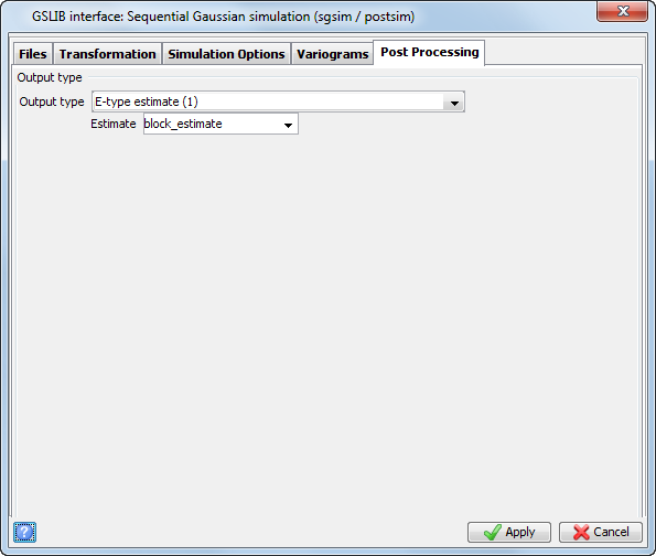
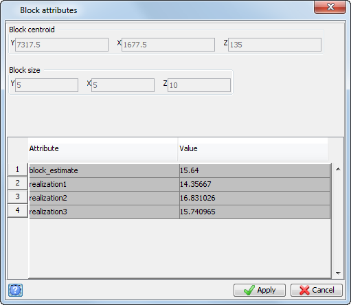
Three new attributes have been created to store each of the simulation realizations, using the name specified on the Files tab (Output - Estimation). In this example, the name "realization" was used. In addition, a block value estimate (E-type estimate) has been calculated and is stored in the attribute block_estimate . The attribute must exist prior to running SGSIM. The E-type estimate is the average of all realizations.
Note: To see each of the steps performed in this task, run 2d_12d_conditional_simulation.tcl .
Task: Display conditional simulation results
- Open gc_simulation_completed.mdl.
- Choose Display > Display block model.
- Enter the information as shown, and click Apply.
- Choose Constraints > New graphical constraint.
- Enter the information as shown, and click Apply.
- Choose Display > Colour model by attribute.
- In the Attribute to colour by field, select realization1, and click Scan, for the Range for colour selection type 0,15;999 and click Refresh.
- Click Apply.
- Display the legend on the Legend tab.
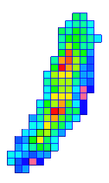
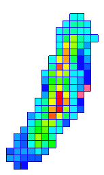
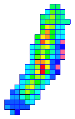
- Repeat the display for realization2, realization3, and block_estimate.
- Choose Block Model > Close.
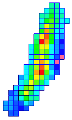
The constrained model is displayed.
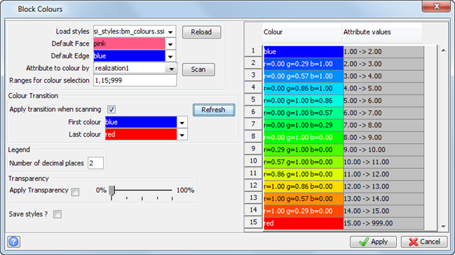
The data and model are displayed, as shown.
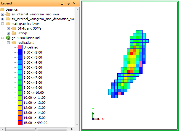
| realization1 | realization2 | realization3 | block_estimate |
|---|---|---|---|
|
|
|
|
Task: Report tonnes and grade for a conditional simulation model
- Open gc_simulation_completed.mdl.
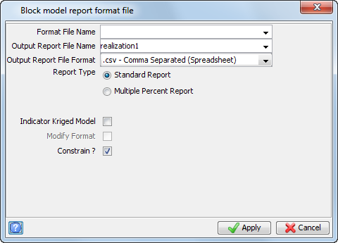
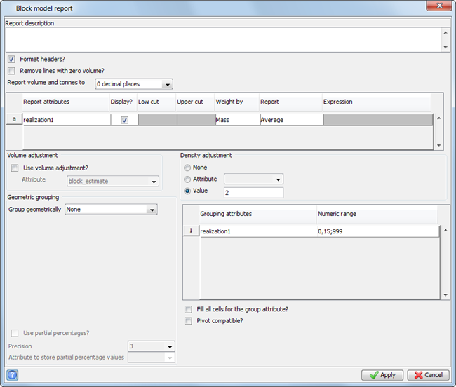
- Choose Block model > Report.
- Enter the information as shown on each of the following forms, and click Apply.
- Repeat the block model report for each realization.
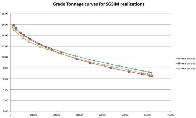
- When you are finished, combine the *.csv files into one *.xls file.
- Open SGSIM_grade_tonnage.xls as an example of the combined reports.
Note: To see each of the steps performed in this task, run 2d_12f_simulation_report.tcl.