Indicator estimation
Overview
Indicator estimation is a useful technique to use when:
- a single geological domain contains two or more populations
- estimation blocks are much larger than mining blocks
- experimental variograms are extremely difficult to model due to small sample size
Indicator estimation is commonly performed using Multiple Indicator Kriging (MIK). MIK is commonly shortened to "IK", or Indicator Kriging, despite the fact that this name is technically incorrect. In accordance with common usage MIK will be referred to as IK throughout the rest of this document.
IK produces a cumulative frequency function (CFF) for each block. After estimating the CFF, the percent of a block above/below a given cutoff can be estimated, which can also be interpreted as the percentage chance that the entire block is above or below a given cutoff.
Although there are advantages to using IK, the amount of work required before you begin estimation is significantly greater than for other estimation methods, such as inverse distance or ordinary kriging. This additional work is commonly cited as one reason not to perform IK. However, for certain situations, such as a mixed populations, IK can be the best estimator, so the extra work is accepted.
You will learn about:
- the indicator estimation process
- choosing indicator cutoffs
- indicator transformation
Requirements
In order to understand this information, you should be familiar with:
- Surpac string files
- variograms
- variogram maps
- the concept of anisotropy
- ordinary kriging
The indicator estimation process
The most common steps to produce an indicator estimation in Surpac are:
- Choose a series of cutoff values.
- Use indicator variogram maps to determine anisotropy ellipsoid parameters for each cutoff.
- Create a block model.
- Perform indicator kriging, using the cutoffs from step 1, and the anisotropy ellipsoid parameters from step 2, to create a Cumulative Frequency Function (CFF) for each block.
- Use the CFF to calculate the overall block value, or percent of the block above or below a given cutoff.
- Report the grade and tonnage from the IK model.
Choosing indicator cutoffs
One method of selecting indicator cutoffs is to use data values which correspond to the deciles of the data (10%, 20%, 30%, ... 90%), as well as some values near the high end of the cumulative frequency to define the "upper tail" of the cumulative frequency function (95%, 97.5%, 99%). In practice, 10 to 15 cutoffs is quite common.
Alternatively, if you know what values will be used for classifying and reporting ore reserves, you can use them as indicator cutoffs. For example, if you know material will be classified into waste, low grade ore, high grade ore, you can use the cutoff values for each of those categories as indicator cutoffs.
Task: Choose indicator cutoffs from percentiles
In this task, you will select cutoff values based on cumulative frequency values.
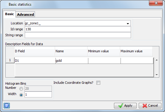
- Choose Geostatistics > Basic statistics.
- Choose File > Load data from string files.
- Enter the information as shown, and click Apply.
- Choose Display > Histogram.
- Choose File > Save as > Image file.
- Enter the information as shown, and click Apply.
- Choose Statistics > Report.
- Enter the information as shown, and click Apply.
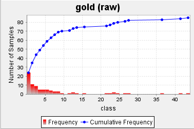
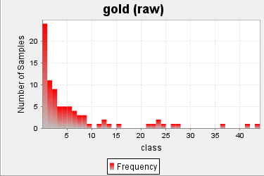
The histogram and cumulative frequency are displayed.
The histogram is displayed
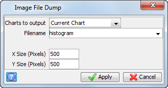
The image is saved in the current working directory.
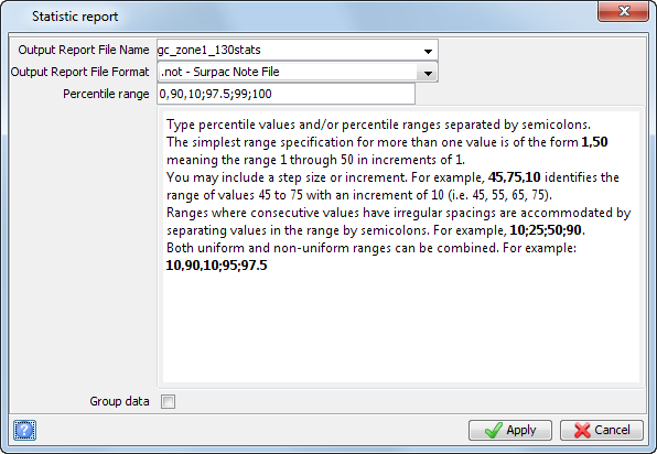
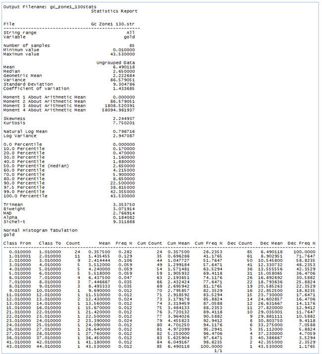
The file gc_zone1_130stats.not is created and displayed.
- Close the Basic Statistics Window.
 Note: To see all of the steps performed in this task, run 2d_02a_basic_statistics_histogram.tcl.
You can use the values associated with each of the specified percentiles as the cutoff values.
| Cutoff number | Cutoff value |
|---|---|
| 1 | 0.17 |
| 2 | 0.47 |
| 3 | 1.16 |
| 4 | 1.88 |
| 5 | 2.65 |
| 6 | 4.22 |
| 7 | 5.90 |
| 8 | 8.65 |
| 9 | 22.5 |
| 10 | 27.2 |
| 11 | 38.82 |
| 12 | 42.36 |
Note: It is not necessary to select a "top cutoff" that is above all data values. When you perform indicator kriging (IK), you can specify a value which is assumed to be the mean value above the last cutoff.
Task: Choose indicator cutoffs from ore classification grades
In this task, you will assume that before you begin creating an indicator estimation, you are provided with the following information:
| Ore Classification | Grade (grams/Tonne) |
|---|---|
| Waste | 0.00 to 1.00 |
| Low Grade | 1.01 to 2.50 |
| Medium Grade | 2.51 to 5.00 |
| High Grade | 5.01 to 10.00 |
| Super High Grade | above 10.00 |
Based on this information, you would choose four cutoffs:
| Cutoff number | Cutoff value |
|---|---|
| 1 | 1.0 |
| 2 | 2.5 |
| 3 | 5.0 |
| 4 | 10.00 |
Note: These values will be used in subsequent tasks because of the small number of cutoffs.
Indicator transformation
After you have determined the value of each of the indicator cutoffs, Surpac transforms all data to a value of one or zero for each cutoff, and then use the transformed values to perform a function. For example, calculating an indicator variogram map or performing indicator kriging. Although Surpac does this transformation for you, it is important to understand how an indicator transformation works.
For each indicator value, a data point is transformed based on the following table:
| If the data value is: | Then the transformed value is: |
|---|---|
| less than or equal to the cutoff | 1 |
| greater than the cutoff | 0 |
Since all data points are either transformed to a value of zero or one, there are no outliers, and the coefficient of variation is small. This means that indicator variograms can be more "well behaved" than normal variograms for data sets that contain outliers or small numbers of data.
Task: Perform indicator transformation
- Open ik_demo.str in Graphics.
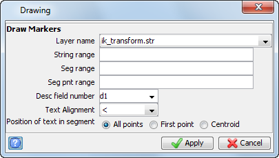
- Choose Display > Point > Markers.
- Enter the information as shown, and click Apply.
- Choose Display > Point > Attributes.
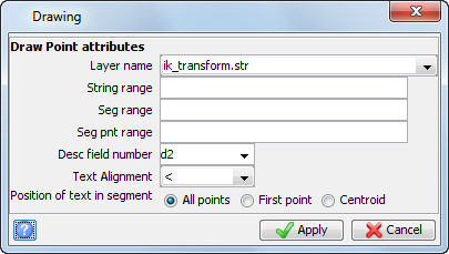
- Enter the information as shown, and click Apply.
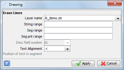
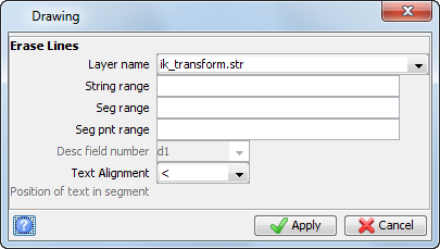
- Choose Display > Hide strings > As lines.
- Enter the information as shown, and click Apply.
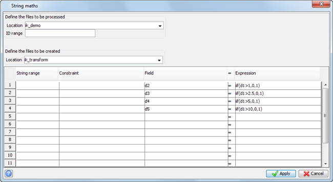
- Choose File tools > String maths.
- Enter the information as shown, and click Apply:
- Click Reset graphics
 .
. - Open ik_transform.str.
- Choose Display > Hide strings > As lines.
- Enter the information as shown, and click Apply.
- Choose Display > Point > Markers.
- Enter the information as shown, and click Apply.
- Choose Display > Point > Attributes.
- Enter the information as shown, and click Apply.
- Choose Display > Point > Attributes.
- Enter the information as shown, and click Apply.
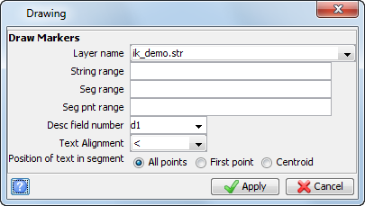
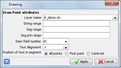
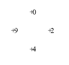
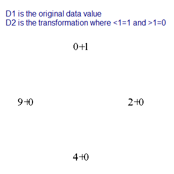
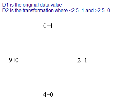
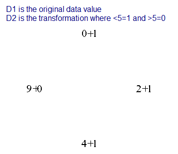
Note: The file contains four points, with D1 values of 0, 2, 4, and 9. These will be transformed to 1 or 0 for each of the four grade classification cutoff values of 1, 2.5, 5, and 10.
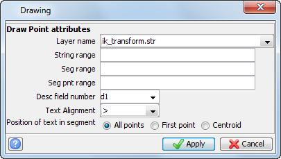
D1 values are displayed on the left of each point marker, and D2 values on the right.
- Repeat steps 20 and 21, selecting a Desc field number of D3, then D4, and then D5.
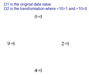
Note: To see all of the steps performed in this task, run 2d_11a_ik_transform.tcl.
Indicator estimation
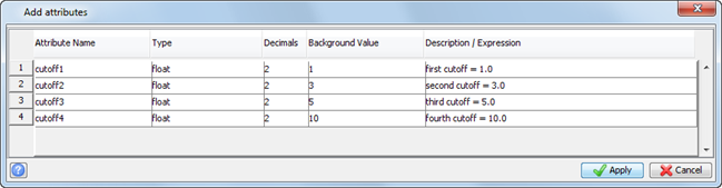
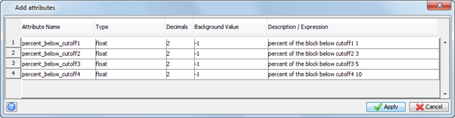
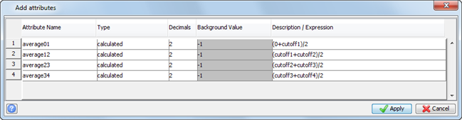
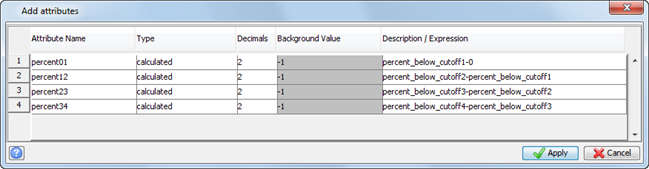
Indicator kriging is used to estimate a cumulative frequency function and block value for a single block from four samples, all equally spaced from the block centroid.
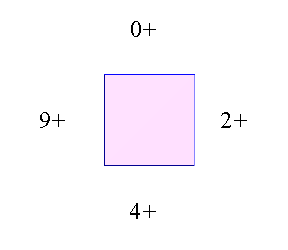
Four cutoff values are chosen from ore classification grades.
| Cutoff number | Cutoff value |
|---|---|
| 1 | 1.0 |
| 2 | 2.5 |
| 3 | 5.0 |
| 4 | 10.00 |
Isotropy is assumed for all cutoffs.
Task: Perform indicator estimation
- Run 2d_11b_indicator_estimation.tcl.
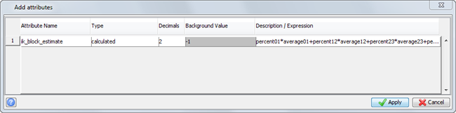
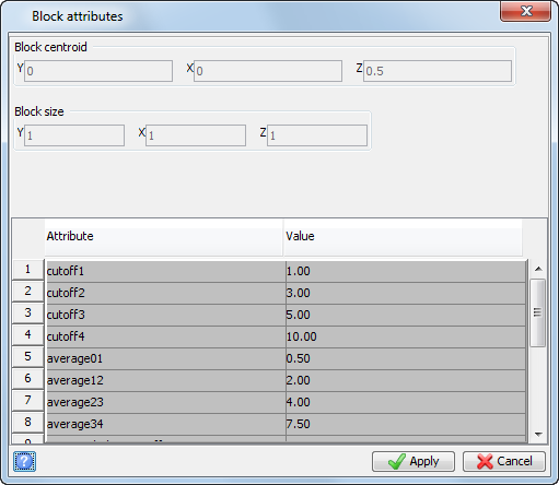
- Click Apply on each form presented.