Indicator variogram maps

Overview

Indicator variogram maps are used in the same way as ordinary variogram maps to obtain anisotropy ellipsoid parameters.  When you create an indicator variogram map, the data is transformed to indicator values based on the value of each cutoff.  The entire process of determining anisotropy ellipsoid parameters is repeated for each cutoff.

You will learn about using indicator variogram maps to determine anisotropy ellipsoid parameters for a series of cutoffs

Requirements

In order to understand this information, you should:

• be familiar with Surpac string files
• know how to create and use variogram maps to obtain anisotropy ellipsoid parameters
• understand the concepts of anisotropy and ordinary kriging

Using indicator variogram maps

In order to create indicator variogram maps, you must have defined a set of cutoff values.  To keep the procedure simple, only four cutoffs are used in this exercise. 

The end product of the process of using indicator variogram maps is to get anisotropy ellipsoid parameters for indicator kriging.  These parameters need to be documented for each cutoff.

Task: Calculate anisotropy parameters for each cutoff

1. Choose Block model > Geostatistics > Indicator variogram modelling.
2. Choose Variogram Map > New variogram map.
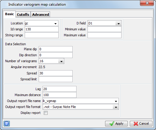
3. On the Basic tab, enter the information as shown.



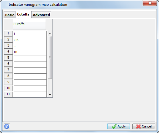
4. Click the Cutoffs tab, and enter the information as shown.



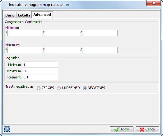
5. Click the Advanced tab, enter the information as shown, and click Apply.



6. Right-click and choose Tile Windows.
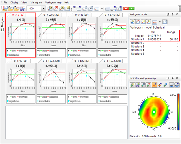
7. Use the variogram map to identify the major axis for the first cutoff (1.000), as shown.
8. Use Variogram > Model to create a variogram for that orientation, and note the Range.
 



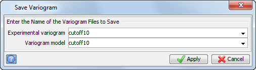
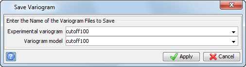
9. Choose File > Save > Experimental variogram and model.
10. Enter the information as shown, and click Apply.



11. Modify the variogram to best-fit the semi-major axis (keep the nugget and sill the same), and note the range.



12. Calculate the anisotropy ratio (range of the major axis divided by the range of the semi-major axis) for the first cutoff:

major/semi-major anisotropy ratio = 60 / 30 = 2

13. Document the values as shown.

Cutoff	Variogram	Bearing	Major/Semi-Major Anisotropy Ratio
1	cutoff10.vgm	0	2.0
2.5
5
10

14. Use the cutoff selectorto display the variogram map for the next cutoff (2.5).



15. Use the variogram map to identify the major axis for the 2.5 cutoff, as shown.
16. Create a variogram for that orientation, and note the Range.
 



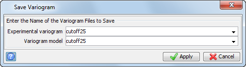
17. Choose File > Save > Experimental variogram and model.
18. Enter the information as shown, and click Apply.



19. Modify the variogram to best-fit the semi-major axis (keep the nugget and sill the same), and note the range.



20. Calculate the anisotropy ratio (range of the major axis divided by the range of the semi-major axis) for the first cutoff:

major/semi-major anisotropy ratio = 75 / 25 = 3

21. Document the values as shown.

Cutoff	Variogram	Bearing	Major/Semi-Major Anisotropy Ratio
1	cutoff10.vgm	0	2.0
2.5	cutoff25.vgm	22.5	3.0
5
10

22. Use the cutoff selector to display the variogram map for the next cutoff (5.0).
23. Use the variogram map to identify the major axis for the 5.0 cutoff, as shown.
24. Create a variogram for that orientation, and note the Range.
 



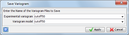
25. Choose File > Save > Experimental variogram and model.
26. Enter the information as shown, and click Apply.



27. Modify the variogram to best-fit the semi-major axis (keep the nugget and sill the same), and note the range.



28. Calculate the anisotropy ratio (range of the major axis divided by the range of the semi-major axis) for the first cutoff:

major/semi-major anisotropy ratio = 68 / 30 = 2.3

29. Document the values as shown:.

Cutoff	Variogram	Bearing	Major/Semi-Major Anisotropy Ratio
1	cutoff10.vgm	0	2.0
2.5	cutoff25.vgm	22.5	3.0
5	cutoff50.vgm	22.5	2.3
10

30. Use the cutoff selector to display the variogram map for the next cutoff (10.0).
31. Use the variogram map to identify the major axis for the 10.0 cutoff, as shown.
32. Create a variogram for that orientation, and note the Range.



33. Choose File > Save > Experimental variogram and model.
34. Enter the information as shown, and click Apply.



35. Modify the variogram to best-fit the semi-major axis (keep the nugget and sill the same), and note the range.



36. Calculate the anisotropy ratio (range of the major axis divided by the range of the semi-major axis) for the first cutoff:

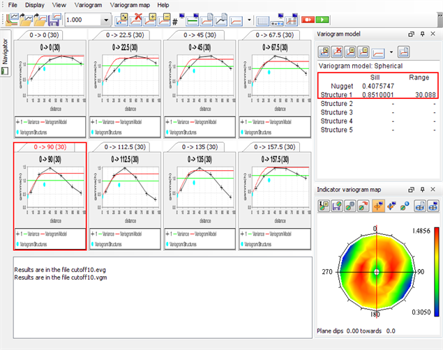
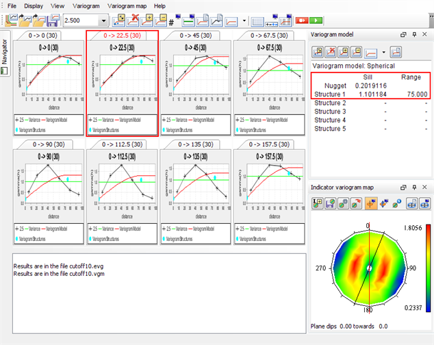
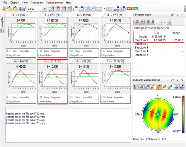
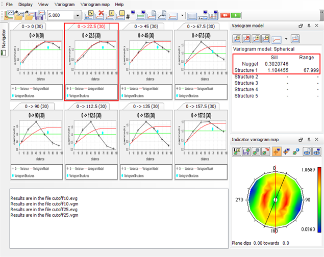
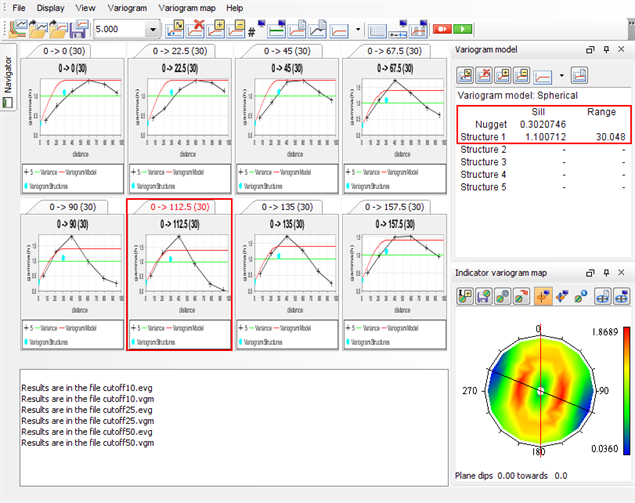
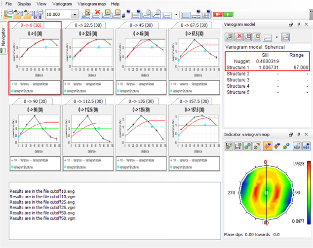
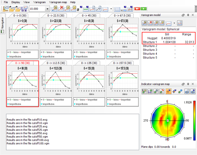
major/semi-major anisotropy ratio = 67 / 32 = 2.1

37. Document the values, as shown.

Cutoff	Variogram	Bearing	Major/Semi-Major Anisotropy Ratio
1	cutoff10.vgm	0	2.0
2.5	cutoff25.vgm	22.5	3.0
5	cutoff50.vgm	22.5	2.3
10	cutoff100.vgm	0	2.1

Note: This exercise, with four cutoffs, demonstrates that the amount of work to obtain the parameters necessary for performing indicator kriging of one attribute (gold, in this case) is equal to four times the amount of work required to obtain the anisotropy parameters for ordinary kriging.  Normally, ten or more cutoffs are used. This means it requires ten or more times the amount of work per attribute. Multiply this times the number of attributes per model, and can see that considerable effort is required to derive all of the anisotropy ellipsoid parameters for all attributes in a model. This extra work is a main reason why indicator kriging is not used for the majority of resource estimations. If a data set contains multiple populations (as evidenced by a bimodal distribution), which cannot be geographically separated, then indicator kriging is used because it is seen as a viable alternative, despite the work involved.