


Inverse distance estimation
Overview
An important end product of a geostatistical evaluation is a “model”, or a set of points in space which contain estimated values. One of the methods for estimating values at points in a model is known as inverse distance estimation.
You will learn about:
- comparing isotropic and anisotropic inverse distance estimation
- the steps to performing inverse distance estimation
- the impact of power on inverse distance estimation
- how to implement anisotropy parameters from a primary variogram map
Requirements
In order to understand this information, you should:
- know how to display menu bars
- be familiar with Surpac string files
- know how to calculate and model a variogram in Surpac
- understand the concept of an anisotropy ellipsoid
- understand the parameters which define an anisotropy ellipsoid
Comparing isotropic and anisotropic inverse distance estimation
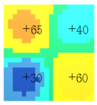
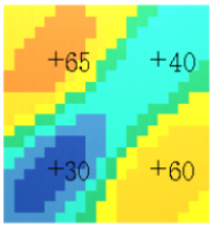
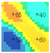
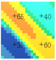
When you use inverse distance weighting to estimate values in a block model, the amount and direction of anisotropy can have a significant impact on the end result. For example, the four models shown below were created from the same data set, but different amounts and orientations of anisotropy were used.
|
|
|
|
No Anisotropy (Isotropic) |
2:1 Anisotropy Azimuth 45 |
|
|
|
|
2:1 Anisotropy Azimuth 135 |
5:1 Anisotropy Azimuth 135 |
Task: Perform inverse distance estimation using isotropy
- Open 4points1.str in Graphics.
- Choose Display > Point > Markers.
- Enter the information as shown, and click Apply.
- Choose Display > Point > Attributes.
- Enter the information as shown, and click Apply.
- Choose Display > Hide strings > As lines.
- Enter the information as shown, and click Apply.
- Right-click in the empty area to the right of the menus and choose Menus > Block Model.
- Open the model 20x20x1.mdl.
- Choose Display > Clear model colours.
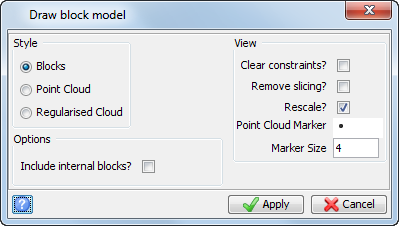
- Choose Display > Display block model.
- Enter the information as shown, and click Apply.
- Choose Estimation > Inverse distance.
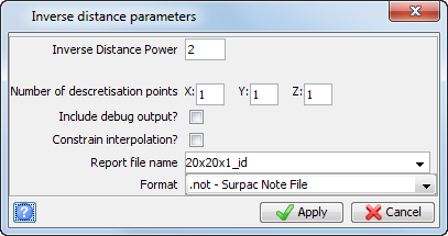
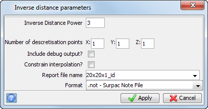
- Enter the information as shown, and click Apply on the following three forms.
- Choose Display > Colour model by attribute.
- In the Attribute to colour by firld, select isotropic, click Scan, then enter values for the Ranges for colour selection of 30,70,5 and click Refresh.
- Click Apply.
- Choose Block Model > Close.
- On the Exit block model form, click Save and exit, and then click Apply.
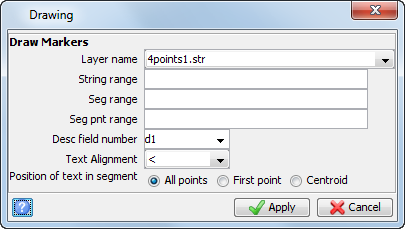
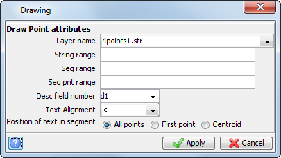
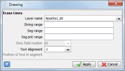
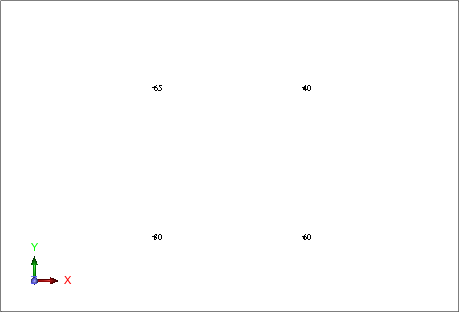
The points are displayed as follows.
 Note: All menu commands below here refer to the Block Model menu bar.
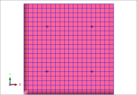
The model and data are displayed.
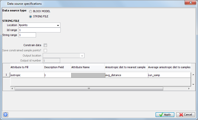
Note: The parameters Anisotropic dist to nearest sample, Average anisotropic dist to samples, and Number of samples are optional.
By filling in the form this way, you specify that the data comes from string 1 of 4points1.str and that the calculated grade will be stored in a block model attribute called isotropic.
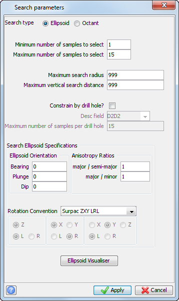
Note: By setting both anisotropy ratios to 1, isotropic estimation will be performed.
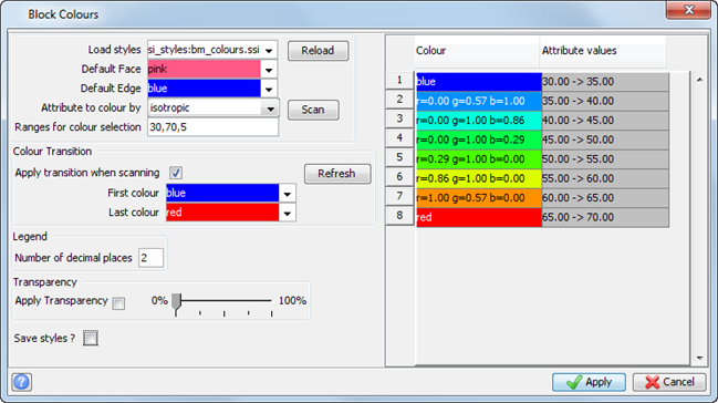
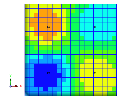
Blocks are coloured based on the inverse distance squared estimate.
Note: To see all of the steps performed in this task:
- Run 2d_04_anisotropy.tcl
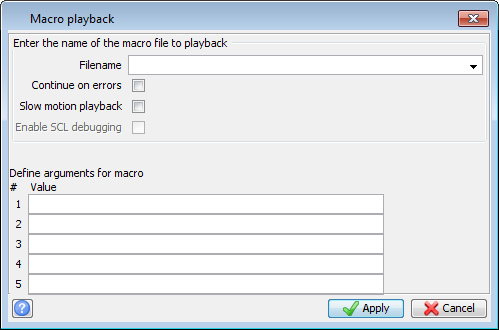
- Use the Macro playback button and select Slow motion playback to display each form.
Task: View the effect of increasing inverse distance power
- Open and display model 20x20x1.mdl.
- Choose Estimation > Inverse distance.
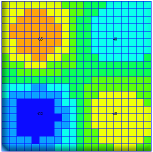
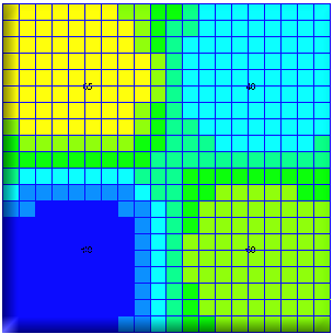
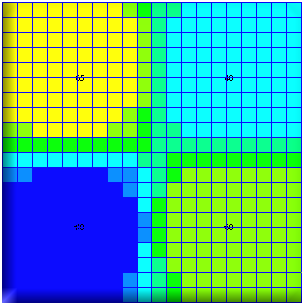
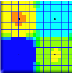
- Enter the information on each form as in the previous task, except for the last form. Instead of an Inverse Distance Power of 2, enter 3, and click Apply.
- Display the model coloured by the isotropic attribute, as described in the previous task.
- Repeat steps 2, 3, and 4 using inverse distance powers of 4 and 10.
- Choose Block Model > Close.
- On the Exit block model form, click Save and exit, and then click Apply.
|
|
|
| Power of 2 | Power of 3 |
|
|
|
| Power of 4 | Power of 10 |
Note: To see all of the steps performed in this task:
- Run 2d_08a_id_power.tcl
- Use the Macro playback button and select Slow motion playback to display each form.
Task: Perform inverse distance estimation on grade control data
- Click Reset graphics
 .
. - Open gc_zone1_cut130.str in Graphics.
- Choose Display > Point > Markers.
- Enter the information as shown, and click Apply.
- Choose Display > Hide strings > As lines.
- Enter the information as shown, and click Apply.
- Open gc130.mdl.
- Choose Display > Display Block model.
- Enter the information as shown, and click Apply.
- Open gc_orezone1.con in Graphics.
- Click Faces off
 .
. - Choose Estimation > Inverse distance.
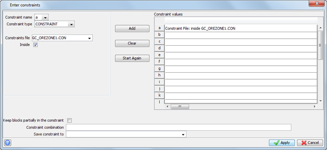
- Enter the information as shown, and click Apply on the following four forms.
- Choose Display > Colour model by attribute.
- In the Attribute to colour by field, select gold_id2, click Scan, and then for the Range for colour selection enter 0,15,1 and click Refresh.
- Click Apply.
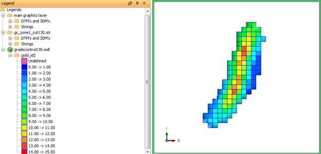
- Display the legend on the Legend tab.
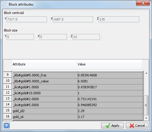
- Choose Attribute > View attributes for one block.
- Click any block.
- Click Apply.
- Choose Block Model > Close.
- On the Exit block model form, click Save and exit, and then click Apply.
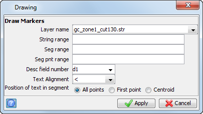
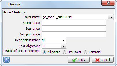
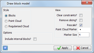
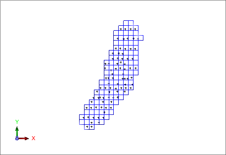
The data and model are displayed.
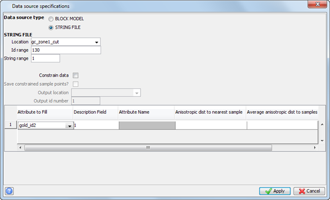
Note: The Anisotropic distance, Average anisotropic distance, and Number of samples fields are optional.
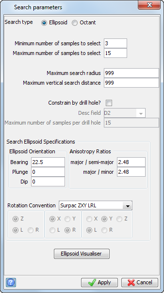
Note: The major axis and anisotropy ratios from the primary variogram map exercise are used here. The major/minor ratio must be equal to or greater than the major/semi-major ratio, even for 2D estimation.
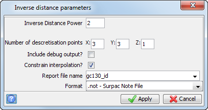
Note: In order to restrict the blocks to the domain "Zone 1", you must select Constrain interpolation.
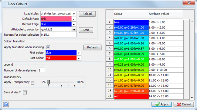
The data and model are displayed:
The value estimated for the block is displayed.
Note: To see all of the steps performed in this task, run 2d_08b_inverse_distance.tcl.