Variogram Concepts

Overview

An important aspect of performing any geostatistical evaluation is to understand how data values change over distance and direction.  A variogram is a graphical tool which can be used to describe these concepts.

You will learn about:

• basic variogram concepts
• variogram calculation
• the impact of modifying the lag distance
• omnidirectional variograms
• directional variograms

Requirements

In order to understand this information, you should:

• be familiar with Surpac string files
• know how to run a Surpac macro
• understand basic statistical concepts such as mean and variance

Basic variogram concepts

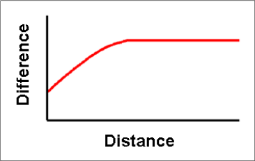
A variogram is a graph that compares differences between samples against distance:

Nugget

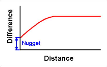
If you split a single sample, and send it to two different labs, very often you will get two different values.  Thus, at a sample separation distance of zero, there is some difference.  This difference is called the "nugget", also abbreviated as "c(0)".  The nugget value is noted as a difference at a sample separation distance of zero:

The term "nugget" comes from a situation that often occurs in coarse gold deposits where a sample is split, and one half contains a gold nugget, while the other half does not contain any gold.  The type of deposit significantly influences the nugget. Gold deposits, with their uneven distribution of metal, usually have a high nugget value. Iron ore deposits, with their fine grains and even distribution, usually have a low nugget value.

Although differences between sample "splits" is often responsible for the nugget, human error can also be a factor.  Errors occur in sampling, in the lab, and during data entry.  Any or all of these can contribute to the nugget.  Although these areas are beyond the scope of this tutorial, you should be aware of them, and their impact on the nugget and subsequent geostatistical evaluations.

Sill

If you compare two samples that are some distance apart, you would expect the difference to be greater than samples which are closer together.  The portion of the graph of the variogram which rises up and to the right of the nugget point, represents this situation. 

At some point, the difference between the samples cannot get any greater.  For example, the maximum sample value minus the minimum sample value gives us the greatest difference between samples.  On the variogram, this maximum difference is displayed as the flat portion of the graph.

Two values describe the point at which the variogram reaches its maximum value – the sill and the range. 

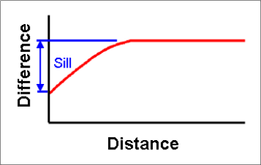
The sill (sometimes abbreviated as the letter "C"), as shown above, is the difference between the maximum difference and the nugget. The term "nugget to sill ratio" is used to describe what percentage of the "total sill" the nugget comprises, and is calculated as:

nugget to sill ratio = nugget / (nugget + sill)

Range

The range is the distance at which the sill is attained.

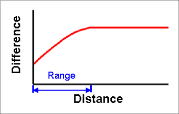
The range (sometimes abbreviated as the letter "A") represents the maximum distance which sample pairs can be said to have some relationship to their separation distance.  Beyond the range, there is no relationship.

Variogram calculation

To calculate a variogram, a data set is grouped into "pairs", which are separated by a given distance, or "lag".  Then the following calculation is performed on all samples in each bin:

gamma(h) = sum of (difference between sample values) squared / 2 x number of pairs

To demonstrate this, you will use the following data.  Assume that the values represent samples taken at 1 metre intervals along a north – south line:

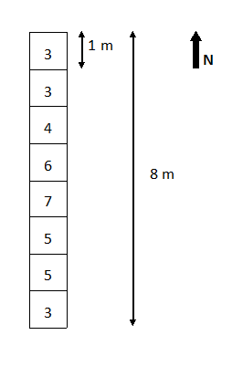
To create the variogram graph of "Distance vs. Difference", you first decide upon a lag distance, or "lag interval".  You then group the data into sample pairs which fall into each lag interval.  For the first lag interval of 1, you get the data pairs of 3-3, 3-4, 4-6, and so on…  The difference between the two values is squared, and the sum of all squared distances is calculated:

Lag = 1
Pair	Pair Values	Difference	Squared difference
1 2 3 4 5 6 7	3 – 3 3 - 4 4 - 6 6 - 7 7 - 5 5 - 5 5 – 3	0 -1 -2 -1 2 0 2	0 1 4 1 4 0 4
		sum:	14

gamma(h) = sum of squared differences / 2 x number of pairs

= 14/2x7

= 1.0

Next, all samples separated by lag distances of 2 are paired off, and the calculation is performed again:

Lag = 2
Pair	Pair Values	Difference	Squared difference
1 2 3 4 5 6	3 – 4 3 - 6 4 - 7 6 - 5 7 - 5 5 – 3	-1 -3 -3 1 2 2	1 9 9 1 4 4
		sum:	28

gamma(h) = sum of squared differences / 2 x number of pair s

= 28 / 2x6

= 2.3

The results of lag distances of 3, 4, and 5 are below:

Lag = 3
Pair	Pair Values	Difference	Squared difference
1 2 3 4 5	3 – 6 3 - 7 4 - 5 6 - 5 7 – 3	-3 -4 -1 1 4	9 16 1 1 16
		sum:	43

gamma(h) = sum of squared differences / 2 x number of pairs

= 43/2x5

= 4.3

Lag = 4
Pair	Pair Values	Difference	Squared difference
1 2 3 4	3 – 7 3 - 5 4 - 5 6 – 3	-4 -2 -1 3	16 4 1 9
		sum:	30

gamma(h) = sum of squared differences / 2 x number of pairs = 30/2x4 = 3.8

Lag = 5
Pair	Pair Values	Difference	Squared difference
1 2 3	3 – 5 3 - 5 4 – 3	-2 -2 1	4 4 1
		sum:	9

gamma(h) = sum of squared differences / 2 x number of pairs

= 9/2x3

=1.5

All of the results and lag distances are then compiled:

Lag (distance)	gamma(h) (difference)
1 2 3 4 5	1 2.3 4.3 3.8 1.5

A graph of the results looks like this:

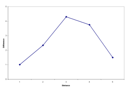
This graph of calculated gamma(h) values versus lag distance is called an "experimental variogram".  This is used to calculate the variogram displayed in the previous version - a "variogram model".  The variogram model can be described by a mathematical equation, and is subject to the interpretation of the person who is analysing the data.  A variogram model, as shown in the previous section, starts at a nugget, increases by the sill at a point defined by the range, then continues infinitely to the right at the total sill value.  A variogram model has been fit to the experimental variogram below:

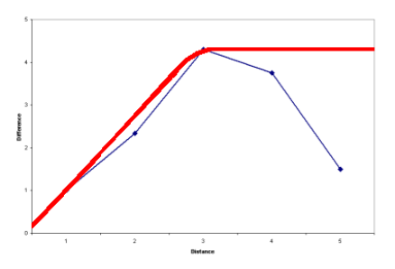
In this example, all relevant parameters of the model would be recorded:

Nugget: 0.2

Sill: 4.0

Range: 3.0

Nugget/Sill ratio = 0.2 / (0.2+4.0) = 0.05

The effect of modifying the lag distance

Although the previous example generated a well-formed experimental variogram, often it is necessary to modify the lag distance to obtain such a good-looking variogram.  In the previous example, a lag interval of 1 was used.  The term "Lag=1" actually meant "all sample pairs whose separation distance is between 0.001 and 1".  "Lag=2" meant "all sample pairs whose separation distance is between 1.001 and 2". "Lag=3" meant "all sample pairs whose separation distance is between 2.001 and 3".

To demonstrate the effect of the value chosen for the lag, you will recalculate the variogram in the previous example, but using a lag interval of 2.  You will calculate three "lag bins": 

Lag=2 sample pairs whose separation distance is between 0 and 2.

Lag=4 sample pairs whose separation distance is between 2.001 and 4.

Lag=6 sample pairs whose separation distance is between 4.001 and 6.

Here is the data again, representing samples taken at 1 metre intervals along a north – south line:

For the 0-2 lag bin, you now get the following data pairs:

Lag = 2
Pair	Pair Values	Difference	Squared difference
1 2 3 4 5 6 7 8 9 10 11 12 13	3 - 3 3 - 4 3 - 4 3 - 6 4 - 6 4 - 7 6 - 7 6 - 5 7 - 5 7 - 5 5 - 5 5 - 3 5 - 3	0 -1 -1 -3 -2 -3 -1 1 2 2 0 2 2	0 1 1 9 4 9 1 1 4 4 0 4 4
		sum:	42

gamma(h) = sum of squared differences / 2 x number of pairs

= 42/2x13

= 1.6

For the 2-4 lag bin, you now get the following data pairs:

Lag = 4
Pair	Pair Values	Difference	Squared difference
1 2 3 4 5 6 7 8 9	3 - 6 3 - 7 3 - 7 3 - 5 4 - 5 4 - 5 6 - 5 6 - 3 7 - 3	-3 -4 -4 -2 -1 -1 1 3 4	9 16 16 4 1 1 1 9 16
		sum:	73

gamma(h) = sum of squared differences / 2 x number of pairs

= 73/2x9

= 4.1

Lag = 6
Pair	Pair Values	Difference	Squared difference
1 2 3 4 5	3 - 5 3 - 5 3 - 5 4 - 3 3 - 3	-2 -2 -2 1 0	4 4 4 1 0
		sum:	13

gamma(h) = sum of squared differences / 2 x number of pairs

= 13/2x5

= 1.3

All of the results and lag distances are then compiled and graphed:

Lag (distance)	gamma(h) (difference)
2 4 6	1.6 4.1 1.3

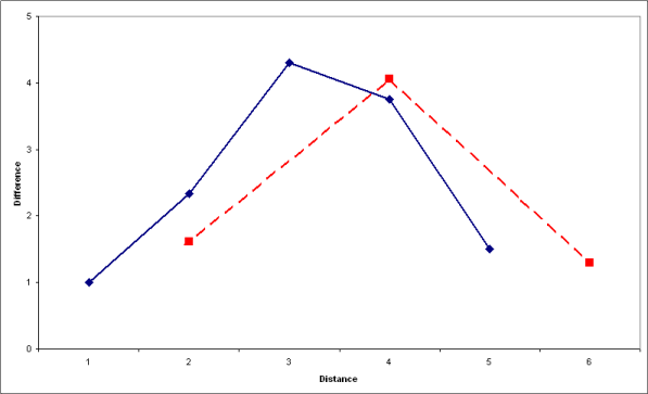
Experimental variograms with lags of 1(solid) and 2(dashed)

Omnidirectional variograms

The variogram in the previous exercise was an example of a "directional" variogram. All samples used were aligned north-south. Another type of variogram is known as an "omnidirectional variogram". In this type, the pairs are selected based only on their separation distance, and not on the orientation of the pairs. 

The example below demonstrates how sample pairs would be selected for a data set. All samples are on a 1x1 grid, and lag values of 1, 2, and 3 are used.  The way in which the software determines pairs is this:

1. Move to the first point.
2. Determine which other points in the data set are within the first lag tolerance distance from this point, and add these pairs to the first "lag bin" (Lag=1).
3. Determine which points not selected are within the second lag tolerance distance from this point, and add them to the second "lag bin" (Lag=2).
4. Repeat until all points have been put into a lag bin.
5. Move to the next point.
6. Remove the previous point from consideration.
7. Repeat steps 2 to 6 until all points have been considered.

In an omnidirectional variogram, the orientation of the sample pairs is irrelevant.  For example, sample pair 1-2 is oriented east-west, sample pair 1-4 is oriented north-south, and yet both pairs are used for the "Lag=1" bin. 

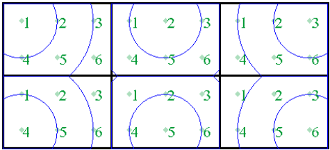
Lag selection circles

Sample pairs selected for each lag in an omnidirectional variogram:

Lag=1	Lag=2	Lag=3
1-2 1-4 2-3 2-5 3-6 4-5 5-6	1-3 1-5 2-4 2-6 3-5 4-6	1-6 3-4

Note: The example here is two-dimensional. In three dimensions, the search from each point takes the shape of a sphere.

Directional variograms

A directional variogram is one in which all sample pairs are oriented in a particular direction.  In the first example, all samples were aligned north-south.  There was no other possible orientation for the sample pairs to take, so the only variogram possible was a directional variogram.

However, in most data sets, there are many data pair orientations.  In a directional variogram, the software selects only those data pairs which are oriented in a particular manner, plus or minus some angular tolerance.  In Surpac, this angular tolerance is known as the spread.

The following example demonstrates how sample pairs are selected for a data set, using a northeast – southwest orientation of 45 degrees, plus or minus a spread tolerance of 22.5 degrees either side of that direction. Thus, if a sample pair is oriented between 22.5 and 67.5 degrees (or 202.5 and 247.5 degrees), it will be included in the calculation. 

All samples are on a 1x1 grid, and lag values of 1, 2, and 3 are used. The way in which Surpac determines pairs is shown below:

1. Move to the first point.
2. Determine which other points in the data set are within the first lag tolerance distance from this point AND within the angular tolerances, and add these pairs to the first "lag bin" (Lag=1).
3. Determine which points not yet selected are within the second lag tolerance distance from this point AND within the angular tolerances, and add them to the second "lag bin" (Lag=2).
4. Move to the next point.
5. Remove the previous point from consideration.
6. Repeat steps 2 to 5 until all points have been considered.

In a directional variogram, the orientation of the sample pairs is important. For example, sample pairs 1-2 and 1-4 are both within the first lag tolerance, but neither are within the angular tolerance of 45 degrees plus or minus 22.5 degrees. In fact, there are only three data pairs in the entire data set which have an orientation that is within the defined limits. These are the data pairs: 2-4, 3-4, and 3-5.

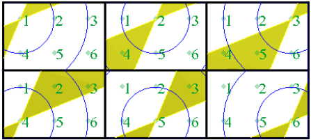
Lag selection circles with directional tolerance search

Sample pairs selected for each lag for a directional variogram (orientation 45 +/- 22.5):

Lag=1	Lag=2	Lag=3
	2-4 3-5	3-4

As you can see, using directional variograms reduces the number of sample pairs.  As the tolerance angle decreases, so does the number of pairs.  If a tolerance angle is too small, the quality of the experimental variogram may be reduced to the point that a model cannot be fitted with any confidence.  If the tolerance angle is too large, the concept of a "directional" variogram could be questioned.

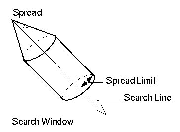
Note: The example here is two-dimensional.  In three dimensions, the search from each point takes the shape of a cone. Additionally, Surpac has the option to restrict the radius of the cone to a maximum using a "spread limit".  This has the effect of turning the search cone into a cylinder with the radius of the spread limit.