


Variogram maps
Overview
An important aspect of performing any geostatistical evaluation is to understand the anisotropy of the data, or which direction has the longest continuity. It is also important to understand how the data values change with regard to the direction with longest continuity, as well as in relation to the two mutually perpendicular directions.
A variogram map is a tool in Surpac that allows you to visualise anisotropy in a plane, and calculate anisotropy ellipsoid parameters to use in estimation.
You will learn about the:
- primary variogram map
- secondary variogram map
- calculation of anisotropy ellipsoid parameters
Requirements
In order to understand this information, you should:
- be familiar with Surpac string files
- know how to calculate and model a variogram in Surpac
- understand the concept of an anisotropy ellipsoid
- understand the parameters that define an anisotropy ellipsoid
Primary variogram map
Task: Create a horizontal variogram map
- Choose Geostatistics > Variogram modelling .
- Choose Variogram map > New variogram map.
- Enter the information as shown on the Basic tab.
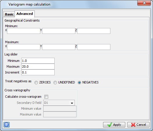
- Click the Advanced tab, enter the information as shown, and click Apply.
- Right-click anywhere on the variogram, and select Tile Windows.
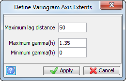
- Choose Display > Set axis limits.
- Enter the information as shown, and click Apply.
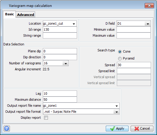
The number of variograms selected will determine the angular increment. In our example, 16 variograms will result in a 22.5 degree angular increment (360/16=22.5). If the number of variograms was set to 36, you would get a 10 degree increment (360/36=10).
The spread and spread limit parameters are the same as in normal variogram modelling.
The relationship between the angular increment and the spread angle should be considered.
It could be considered unreasonable to define a spread tolerance anything greater than half of the angular increment. For this data set, because of the small number of pairs, if a 11.25 degree spread were used (half of the 22.5 degree angular increment between adjacent variograms), the number of data pairs would be so small that very few, if any reasonable variograms would result. A spread of 30 degrees is used for this data set to ensure that enough samples are included to produce meaningful variograms.
Given that a spread of 30 degrees is used, you could argue that the number of variograms should be reduced to minimise the “overlap” of the cones for adjacent variograms. Although this is a reasonable argument, the resulting variograms would not be suitable to use to use to visually determine anisotropy.
It is up to you, based the data set you are working with,to determine the values you will use to produce a usable variogram without over-smoothing your data. This is an example of how geostatistics is an inexact science. Experience with a data set will usually allow you to determine what combination of parameters will give an acceptable result.
In the bottom panel, the lag, maximum distance, and variogram report parameters are specified, exactly as they are in variogram modelling. One thing you should consider is that the maximum distance will be the radius of the variogram map. You might find that you need to try a few variations of this value to get one that gives an adequate result.
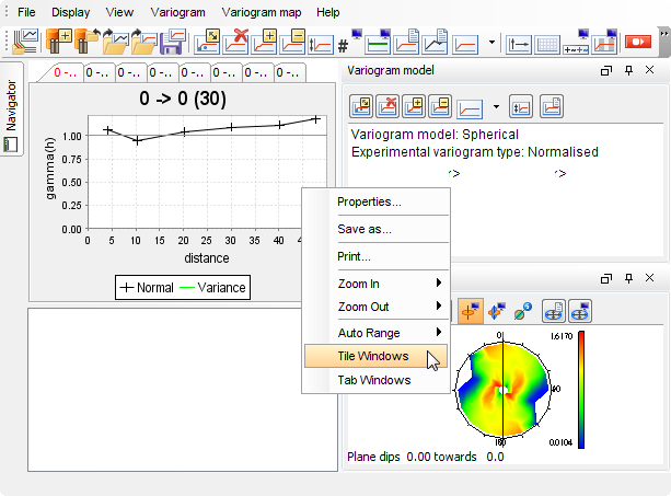
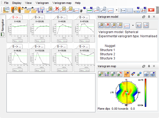
The variograms are displayed.
Task: Determine 2D anisotropy
In a 2D case, both the major and semi-major axes will lie in the plane of the primary variogram map. The orientation of the major axis is chosen as the variogram which has the longest range for a given sill value.
- Move the lag slider back and forth, changing the colours in the variogram map to show you areas of high and low variance .
- After you have an idea of what appears to be the orientation of the longest range, use the lag slider to improve the quality of the experimental variogram for that direction. In the previous image, a lag distance of 4.3 resulted in a good variogram for the 45 degree orientation.
- Choose Variogram > Model.
- Click and drag the model to fit the experimental variogram for that direction.
- Check that variogram model for all other orientations.
- If another orientation appears to have a longer range and a lower variance, modify the model to fit that experimental variogram.
- Modify the variogram for the orientation of 22.5, as shown below.
- Repeat the previous two steps until you are satisfied that you have the orientation of the major axis.
- After you have defined a major axis, ask yourself, and others who are familiar with the geology, if the orientation appears correct.
- Choose File > Save > Experimental variogram and model
- Enter the information as shown, and click Apply.
- Choose Variogram > Model.
- Click and drag the variogram so that it fits the experimental variogram for bearing 112.5.
The colour bar at the side of the variogram map shows you the range of variance for your data. You will most likely see that throughout a range of lag values, there will be areas on the variogram map which will be consistently high, and others which will be consistently low. Using the example given above, the orientation of 45 degrees consistently displays colours representing low variance.
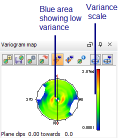
 Note: You are looking for the lag that gives the lowest variance at the centre of the variogram map.
Note: You are looking for the variogram with the longest range for the lowest sill.
This creates a variogram model for the chosen orientation.
As shown below, fit a model to the 45 degree orientation.
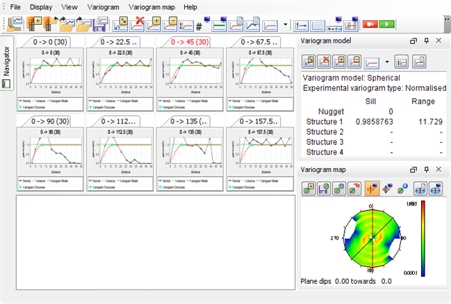
The major axis should be that variogram which has the lowest variance for the longest distance. In this case, the variogram at the orientation of 22.5 degrees actually has a longer range.
Modifying the lag distance for that orientation might help you get a better fit.
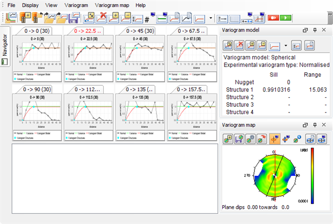
In this case, the orientation of 22.5 is a good match with the orientation of the ore zone as shown below.
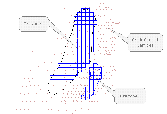
For the ore zone #1, the bearing of the major axis is 22.5.
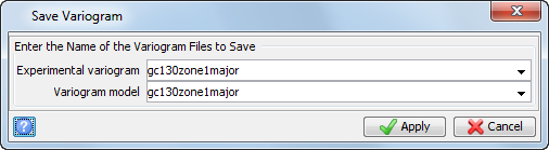
As you can see, not only is the subject of variogram modelling a non-scientific process, but the orientation of the major axis is also open to interpretation and debate.
The semi-major axis is in the same plane, and is perpendicular to the major axis. Thus, the bearing of the semi-major axis for this data set is 22.5 + 90 = 112.5.
The anisotropy ratio is the range of the major axis / range of the semi-major axis for a constant sill value.
The range of the major axis is displayed as 15.1 in the upper right corner of the variogram modelling window.
You can determine the range of the semi-major axis for a variogram with only one structureby changing the range to fit the variogram for the semi-major axis the while keeping the sill the same.
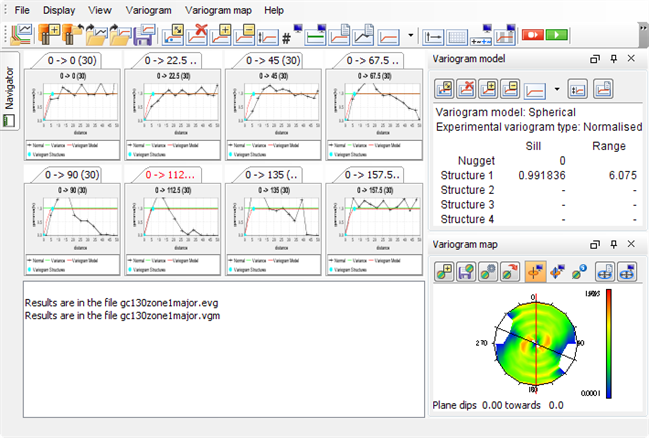
Note: The sill of the variogram is exactly the same, but the range is now 6.075.
Thus, the anisotropy ratio for zone 1 is: 15.1 / 6.1 = 2.48.
Although this is not the purpose for which these functions were designed, this is the quickest means of determining two dimensional anisotropy.